HaRQ: How can I model the growth of a planet's worth of simplistic trees (so \(10^{12}\) trees) fast enough to be useful on a game server?

My hack used walking a Hilbert Curve to order the border crossings of the circles used to denote each tree's sun-collecting area and then building work lists that grow (pun intended!) sufficiently slowly ( so “≤log(N)” ) to maintain a viable maximum memory size.

Overview of the Model Problem

We'll start with the most simplistic setup: There's only one resource, sunlight; all the trees are hemispherical, everything can be projected down onto a 2D surface; and with a tree described by its location on a square 2D grid (\(\vec{x}\)), its type, and a single variable (\(r\)) - its size.

The model is also a simplistic energy balance model: amortized over some period of time the change in size is proportional to the net available energy: \[\Delta r \propto \Delta Q\] where \(\Delta Q\) is the amount of energy left over after collecting sunlight and supporting the tree. We can, and should, also write this as a differential equation \[ \frac{d}{dt}r = \xi \frac{d}{dt} Q = \xi P_{net} \] where \(P_{net}\) is the net amortized power \(P_{net} = P_{in} - P_{out}\), and then use the usual tools for doing the numerical integration.

Next, we'll assume the amount of power collected across the surface of an unshaded tree \(P_{in}\) and that used to support its volume \(P_{out}\) are functions of \(r\) alone (NOT location), where the functions are defined by the tree's type. We'll restrict \(P_{in}\) further by saying it's a function of a circular area proportional to \(r\).

Lastly, we'll assume that big trees always shadow little trees, and that any power not collected is missed and is passed onto the next tree down. Since the functions are not dependent on location, they must be constant on regions, that is, \(P_{in}\) only changes on the boundaries where shadowing changes. For example, three trees might be arranged like this :

Which also nicely shows the five collecting regions caused by the shadowing of the larger tree over the other two.

(Note, I've modified these requirements slightly, knowing the solution presented here, to hopefully streamline things a bit.)

Thoughts on Solving

The difficult part of this model is computing \(P_{in}\) for each tree. We need to know the overlaps and the effect of those overlaps.

The first two ideas were :

1. If we assume each tree at its maximum size, we can pre-compute a graph of which trees overlap, then in each time step iterate over all trees computing the actual boundaries.
2. We could render each tree onto a 2D image or canvas, then iterate over the whole image to compute the function in a two pass process.

Both of these ideas have memory, and computational issues. The first has an " \( O(N^2) \) " problem pre-computing the graph (remember we're shooting for \( N=10^{12}\) and it isn't obvious how to walk the graph in such a way that partial results can be cached without effectively holding the whole problem in memory. The second requires a 2D image canvas where many pixels need to be processed and the shadow ordering needs to be stored on each pixel.

My Hack

What would be nice is some way to order the calculations into work lists where partial result caching takes care of itself.

Enter the Hilbert Curve and Hilbert Indexing.

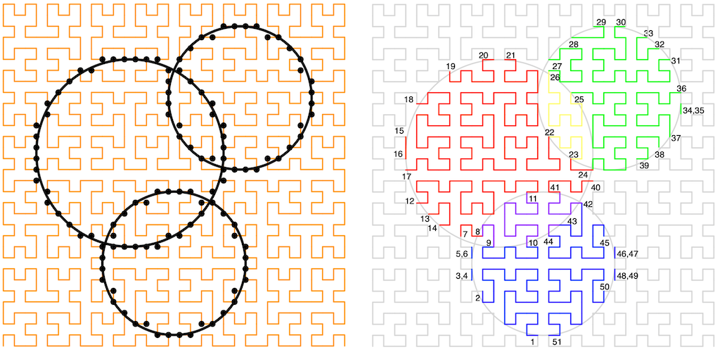
The Hilbert Curve [Future REF] has a useful property: If you walk a Hilbert curve that covers some (square) sub-plane that also contains a bounded region, where the start and end of the Hilbert curve are not inside that region then, as you walk the curve, it will alternately enter and leave the bounded region, until it leaves and never reenters. If we measure the distance from the start of the curve to these crossings and put these measurements into a list, then this walk splits the 2D plane into a list of non-overlapping, monotonically increasing, 1D bounded ranges along the curve. Each list entry will pair up with a neighbor to give a range that is either entirely inside or entirely outside the bounded region. Additionally, the Hilbert Curve is space-filling, so reassembling all of the ranges that are inside the bounded region would cover the entire bounded region.

However, when actually implementing this (as in the figure above), we have to pick a scale and deal with a few edge cases that include when the curve effectively touches, but doesn't cross, the boundary. The monotonic ordering property remains, though.

Here's the rub (part 1): If we pick a scale and are careful with the grid, then there is a mapping from any point on the Hilbert curve on that grid to the distance that point is along the curve [Future REF]. When using a discrete grid like this, the distance along the curve is called the Hilbert Index (of a point). Now, instead of walking the Hilbert curve to find the boundary, we could instead walk the boundary to find all of the XY points on the curve, convert them to their index, and then recover the monotonic range list simply by sorting them! Again, taking neighboring pairs of list entries will give us all the ranges internal to the region (internal ranges), or alternatively external to the region (external ranges).

The length of each of the internal ranges, at whatever grid scale we're using, is the number of grid points, and so grid squares, on that part of the curve inside the region. The sum of all these lengths gives the total number of grid squares inside the region, which is exactly the area of the region (again, from the space filling property). This works for any shape of region, not just the circle shown.

Here's the rub (part 2): If we have the monotonic list of ranges for two bounded regions, we can combine them efficiently with a merge sort. If the regions do not overlap, then the resulting internal range pairs will remain intact as the curve has to leave one region before entering the other. If the regions do intersect, then we have to be a little more careful as we'll have indexes both for when the curve enters or leaves a region but also for when the curve enters or leaves an overlap. So, for our three overlapping tree example:

With a little bit of care and tracking, we can turn a list of overlapping trees into a list of region boundaries and then into a list of ranges that will allow us to compute the area of the shadows and shadow overlaps easily, no matter what those overlapping shapes look like.

From our assumptions, the value of \(P_{in}\) is constant over these regions, so we can compute the total \(P_{in}\) for each tree by doing the appropriate computation on each range pair, that is, by doing computations on the boundaries, not over the area. While while the computation isn't \(O(1)\) with respect to \(r\), it should be a less than \(O(r)\) depending on how and what calculations are cached, and it nowhere near \(O(r^2)\).

As a side note this is closely related to other Boundary Element Methods and things like the Generalized Stokes' Theorem, more on that in another post, but here we'll use the fairly naive way I first built things.

The Algorithm Part 1 - Streaming Lists

We'll ignoring parallelism for the moment, and the integration part, and start by looking at computing the derivatives, that is, the value of \( P_{net} \), or more importantly \(P_{in}\).

First, we need to know which trees should be 'active' as we walk along the curve. Let's assume each tree has a maximum \(r\) value of \(r_{max}\) and walk that radius boundary for each tree: there will be a smallest \(I_{min}\) and largest \(I_{max}\) index value from when the curve first enters and last leaves the tree's region. We can then pre-build a list of data objects that contain the data space needed for each tree, along with the \(I_{min}\) and \(I_{max}\) values, sorted on the \(I_{min}\) value. This initial list is in ascending \(I_{min}\) order. We'll call this list the Initial Points List (IPL).

From the Hilbert curve's perspective, we want to walk along the curve, activating a tree at its \(I_{min}\) value and deactivating it again at its \(I_{max}\) value, because after that, the curve can never return to that tree's region.

From the IPL's perspective, this process is a fold over the list, adding each tree at the head of the list to our set of active trees, and carefully deactivating any tree whose \(I_{max}\) is smaller than the head's \(I_{min}\). As a tree is deactivated, and we are finished with it for now, we can push it onto the head of an output list.

This output list will be in descending \(I_{max}\) order, and with a little care, it should come as no surprise that our algorithm is overall agnostic to which end of the curve we start walking from, so we can use both ascending and descending orderings equally well without having to reorder anything.

So, we start off ordering the tree objects into an IPL, which lets us stream them into our computation algorithm, which will then stream out finished tree objects in the opposite but equally usable ordering, ready to be the IPL for the next pass through the data.

The Algorithm Part 2 - Doing the Work

To reiterate, if our list is ascending, then trees A and B with \(A.I_{min} < B.I_{min}\) cannot interact if \(A.I_{max} < B.I_{min}\) because there are no overlapping ranges. Similarly, if our list is descending, then trees A and B with \(A.I_{max} > B.I_{max}\) cannot interact if \(A.I_{min} > B.I_{max}\) for the same reason.

We'll need another list for the boundary points of regions from active trees using their current \(r\) values; let's call it the Boundary Points List (BPL).

Activating a tree involves walking its current circular boundary based on its current \(r\) and inserting those boundary ranges into the BPL. All of those ranges will be between the \(I_{min}\) and \(I_{max}\) values for this current tree, and the same condition as above applies here too: the current tree's ranges cannot affect any ranges already in the BPL that have an index values less than this \(I_{min}\) value. This means we'll be able to fully process all ranges in the BPL up to the current \(I_{min}\) value.

For the tree being activated, we also need to compute the actual value of \(r\) we'll be using (see the integration section), its shading priority (which is just \(r\)), the capture factor \(\lambda\), and the miss factor \(\mu\).

Schematically, adding the red and green trees from figure 3, the lists will look something like :

To process the ranges, we do the same as before, just in the BPL, that is, we walk the ranges in the BPL, while keeping track of which trees are involved in which range, the ordering stack of tree shadows, while calculating the contributions of each as we go. Fortunately, there are only ever a handful of trees shading a specific, region so the shadow stack will be small, and calculating the ordering isn't expensive.

For a range with index values \( (a,b) \), the \(i^{th}\) tree in our stack of shadowed trees (where zero is the top and sunlight) the contribution to \(P_in\), which we'll call \(p\), is :

\[ p_i = (b-a) \lambda_i \prod_{k=0}^{i-1} \mu_k \]

That is, \(p_i\) for a tree in the current range is the product of the length of the range, its capture coefficient, and all the miss coefficients above it. In practice, we can loop over the stack of trees, keeping track of the current miss coefficient and accumulate \(p\) directly into the tree's data structure.

Deactivating a tree doesn't require any more work on \(P_{in}\) because we know all ranges must have been processed before getting to \(I_{max}\). So, we just need to compute \(P_{out}\) and \(P_{net} = P_{in} - P_{out}\) and bundle up the data structure for output.

The Algorithm Part 3 - Integrating.

I used a standard order 2 Runge–Kutta (so Heun's, Ralson's, or the Midpoint methods). I'll talk about these in detail elsewhere [Future Ref]. For now, we just need to know that RK methods usually proceed in the following way :

1. Compute a derivative at the current input point
2. Compute a trial point from the information we have so far, and compute a derivative at that point.
3. Compute another trial point from the information we have so far, and compute a derivative at that point.
4. ...
5. Compute the full step to the next input point using all the information we have so far.
6. rinse, repeat.

However, since we're streaming the derivatives through lists, and it's going to be a while before we get back to any one point! We need a way to transpose this procedure.

Fortunately, computing a trial point, and computing the full step are closely related, and we can elide step 5 into the next step 1 without much trouble. Now all steps look the same, with the principal difference being that the \(r\) value is only updated on a full step, along with resetting all the trial derivatives to 'not-yet-known'. The downside that the latest \(r\) value won't be known until the next derivative is computed.

Using RK2 means that all ascending walks were computing the derivative at an intermediate trial point, while all descending walks were computing the derivative at a full step.

Lastly, I used only an order 2 method, and instabilities happen, always, especially at low orders. So, the \(p\) values were always clamped, as was the value of \(r\) (to \( 0\le r \le r_{max}\).

Implementation

... was painful!

Mostly because of edge cases arising from using real (discrete) curves instead of the theoretical continuous ones; all the strict inequalities can now sometimes be equalities where the curves touch rather than cross. When this happens, sometimes the correct thing to do is ignore the point, other times it's better to double up the point to make a zero-length range.

Additionally, large datasets took a long time to assemble and test, leading to painfully long debugging cycles for some bugs and edge cases. The initial proof-of-concept code was written in OCAML, but I switched to C++ to gain better control over memory and I/O operations, which made things harder.

It's been a long time (2012) since I ran the full code, and the project was dropped before I was really able to collect much data and prove everything was 100% stable. However, once spun up, the code rapidly becomes memory bandwidth bottlenecked, even for fairly complex energy functions, and some things were repeatedly recomputed on ranges. This implies that memory or cache bandwidth was valuable enough that recomputing rather than memoizing was preferred.

Memory space unexpectedly wasn't a problem. I expected the space requirement and the growth of the BPL to be something like \(O(N^{\frac{1}{2}})\) given we're converting an area problem to a line (boundary) problem. However, to my surprise, \(O( log(N) \) fit much better, but again, not enough data.

In terms of overall speed, the single-threaded code, on a (nice) desktop machine (in 2012), was surprisingly constant, processing around a million ranges per second on average, for a million-tree forest. So, a little over 100,000 trees per second, which it then needed to do twice per time step.

There are around \(3 \times 10^{12}\) trees on earth [Crowther2015]. This would work out at around 1000 days per time step on my 2012 desktop! A modern AMD Threadripper (say the 7995WX) has 96 cores and 8 channels of memory, which is also 4 times faster. Badly extrapolating by assuming memory bandwidth remained the bottleneck, would make it around a month per time step. Not too bad...

Additions and Fun Improvements

So far, there is only one resource (the sunlight at the top of a shadow stack), and it's globally constant. However, there's no reason why these regions we've computed need to be tree shadows. They could also indicate resources directly. For example, a water table or river, or the local(-ish) amount of sunlight given the cloud conditions. They could also be used to include modifications from a [game] designer or player.

There's also no reason the regions need to start circular.

Parallelization was done by splitting the trees into non-overlapping forests and having separate lists for each. I wanted to look at other things:

When processing the BPL up to a new \(I_{min}\), the calculation done on each range is independent of other ranges, so apart from the final accumulation operation, it should be possible to parallelize (farm) them. It's not clear if the benefit of having some local-ish values cached would outweigh the additional management compared to just having enough forest lists.

It should be possible to daisy-chain output lists immediately into another compute unit without storing it first, but it gets complicated. Again, it isn't clear if the benefits would outweigh just having enough forest lists.

Starting with separate forest lists always seemed like a bit of a cheat. I think there might be a way of analyzing the empty ranges in the initial IPL to spot when clumps will never overlap and generate these lists automatically.

The \(P_{in}\) function is very restricted in that it has to be approximated as constant over a region. I hope sometime I'll come back and do the more formal work to prove this out as an actual Boundary Element Method and hopefully reduce the restrictions on \(P_in\).

This was all done while quite deliberately ignoring rendering or any other use for the data. When thinking about rendering, it would be nice to add in lots of things. For example, keeping track of the peak \(r\) values, and using the current-to-peak delta to spot winter die-off and drop leaves, or if the delta is large, have entire dead boughs.

... I have to stop .. every time I come back to this I come up with new things I could do! Feel free to add to this list with a comment or note or something.

Conclusion

My hack was to convert a huge area map problem into a list of lines problem that could then be repeatedly streamed through an integration computation without blowing up memory usage. Each individual calculation on the list is simple with just a few tens of floating-point operations and a few pointer reassignments. The tree model is also very simple; it's just an energy balance on a single variable. The proof-of-concept code was entirely memory bandwidth bottlenecked but still fast enough to put simplistically modeling every tree on a (real) planet within reach.

.... while completely ignoring how one might make use of such a model. Seriously, do you really need \(10^{12}\) trees in your game world ?

Final words

This remains one of my favorite all time projects, and I hope sometime I get to go back to it, as there's a lot of ways to expand and play with it. However the code was not implemented under anything resembling an open source license. Maybe if there is every enough interest I'll re-write and release it, for now here's the python code used to generate all the figures on github

If you like what I do consider subscribing!