A Compression View of Large Language Models

"...extending a prompt with a controlled, often zero, amount of additional random entropy per symbol."

Introduction

I often hear LLM generators described as "just statistical—they can only regurgitate what they've seen!" or, slightly better, "auto-complete on steroids." These descriptions imply that an LLM is just guessing or randomly picking words from a distribution when, in fact, the LLM itself does neither of those things. These descriptions miss the salient detail that an LLM calculates a prediction more akin to how a weather forecast calculates the predicted path of a hurricane; probabilities are still important, but the path isn't a guess.

To explore this idea and show how prediction isn't 'just statistics', we'll need some ideas from Information Theory, and I think a good way to bridge the connection is by building a compression tool with an LLM at its heart.

We'll start with a crash course in compression, then build the LLM-based compression tool, and then explore what it can tell us about the information in text, its predictability, and how to generate seemingly creative text.

Ideas from Compression

The amount of information required to describe something precisely is typically far less than the potential information that could be packed into the space it occupies. This idea underpins the field of data compression, where the goal is to maximize the ratio of relevant information to the data space it consumes. That "typically" is doing some heavy lifting. Not all data can be compressed, and a practical compression tool needs to know or assume something about the information in the data and build that knowledge into the compression tool to be effective.

In the tool we'll build, this knowledge will come via the impressive predictive capability of an LLM, but before we discuss that, we'll need a crash course in how a huge class of compression techniques work.

For the purposes of this article, we'll shoehorn all compression algorithms into a three-part factorization: a Model Module that knows and can predict things about the information being compressed; a Statistical Module that tracks the usage of symbols after the predictions have been accounted for in the data; and an Encoder Module that can use those statistics to pack output symbols as efficiently as possible.

In real applications, things rarely factor this cleanly; modules might have boundaries that overlap or do nothing. However, thinking about any compression algorithm this way is useful for highlighting assumptions about the information being compressed and how that information is separated and moved around.

We'll look at these modules in reverse order.

The Encoder

The purpose of the encoder is to produce a compact representation of data for storage or transmission. In principle, it has two inputs: some structural or format information about the data, and the data itself. However, it is completely agnostic to what that data is, and any contextual information has to come in via the structural information.

For example, consider a date-time string: "17th Jul 11:44:04 PM". This is nicely human-readable but takes up 160 bits of space, much of which is structural and used to present the data in this standard readable form. If we lift this formatting from the string we get a far more compact 80-bit string: "1707234404".

The concept of lifting will recur throughout this article. Lifting is the process of separating or extracting patterns, knowledge, or structure from data, leaving behind the parts that don't conform. It's a reversible, lossless process, meaning you can recombine everything to recover the original form.

In our date-time string we know the valid range of values and boundaries for each field (day, month, hour, etc.), and we can lift this structure out of the data as well. The method to do this is exactly the same as we use for constructing decimal or binary numbers from their written representations: in base 10, we'd construct \(392\) as \( (((3 \times 10) +9) \times 10) +2 \); in base 2, we'd construct \(5\) as \( (((1 \times 2) +0) \times 2 + 1\). For our date-time fields, we construct: \[ ((((17 \times 12) + 7) \times 24 + 23) \times 60 + 44) \times 60 + 4 = 1,424,644 \] This is a variable-base encoding. Each field is encoded with a base just large enough for its values. Each value in a field is now a single symbol in a string of symbols representing a whole number. The largest number we could make doing this would be: \( 31 \times 12 \times 24 \times 60 \times 60 - 1 = 32,140,799 \) which is the last second of the year and fits in just 25 bits.

Note this isn't the same as encoding the date-time as the number of seconds from the start of the year. That would do slightly better, if the year value was known, as the translation to and from the date-time representation would know about leap days and leap seconds, but that is starting to stray into using information beyond the simple structure of the data.

In the above numerical expression, ~96% of all the possible values that fit in 25 bits are valid date-times. Whereas for the 160-bit human-readable string, just \(10^{-40}\) of the possible values are valid—a number so small it's meaningless. To fix this, we usually quantify these sizes on a \(\log_{2}\) scale in units of bits. The human-readable string is 160 bits, while the maximum number from the above expression gives \(\log_{2}(32140799) \approx 24.94\) bits. Note this is not a round number of bits, and we can say, "the 160-bit human-readable string contains less than 24.94 bits of information."

This use of a variable base is a core idea in the arithmetic or range encoding used in many modern compression systems like bzip. For the rest of this article, I'm mostly going to ignore the actual bit encoding. I've lingered on it here as it introduces some useful concepts, specifically how the same information can be contained in different representations of different sizes, that knowledge about the informational structure can be "lifted" out of the data, leaving a compact representation behind, that symbols are just a value-in-a-field, and information sizes measured in bits don't have to be round numbers.

The Statistical Bit

In the last section, each possible value to be encoded was treated as equally likely. However, in general data, this is usually not true. We can use statistics about the occurrence of symbols gathered globally, or at least over some large window, akin to the structural idea above, by encoding more probable values or input symbols with shorter output symbols and rarer input symbols with longer output symbols.

For example, Morse Code uses the general statistics for the English language to encode the commonly used "E" as a single dot, while the less common "O" is three dashes.

Just like with the encoder above, local context is ignored. Morse Code doesn't care, and doesn’t change, if your message is well-formed English or a string of Os.

Of course, we can do better by collecting statistics about the symbols in the actual data being compressed. Computing, tracking, and providing these statistics to the encoder is the job of the Statistical Module in our factorization.

For the tool we're building here, these statistics will be a simple histogram of the data passed into this module. More complex systems might expect and track a probability distribution from the predictive module discussed below, but in general, it is the actual post-modeled data that is important, not how well the model thinks it is doing.

For a fuller explanation of how these statistics are used to efficiently pack output symbols into an output stream, refer to Robert Bamler's paper Understanding Entropy Coding With Asymmetric Numeral Systems (ANS): A Statistician’s Perspective. The code we'll develop later in this article will use the ANS coder from this paper almost exactly.

The next step is to look at context, which brings us to modeling and prediction.

Predictive Modeling

The idea here is that many real-world systems, including language, are highly predictable. This is not a statistical thing; it isn't a guess from statistical distribution; it is calculating how a system will change. If we can make accurate predictions about how a data stream will change, then we can lift or subtract those predictions from the data, leaving behind data that is, in some sense, smaller because it no longer contains that predictable information.

For example, gzip can compress Western text quite effectively. However, if you apply a simple transformation—flipping the case of the first letter after every period—the resulting file will compress very slightly better. This is because the number of symbol types gzip sees is smaller, as it doesn't need to track two versions of words like "The" and "the." Without this transform, gzip doesn't know there is any relation between these two. To decompress, you simply apply the same transformation again after ungzip, since it's an involution, to recover the original text.

If we apply this to the same text we'll use later in the example section and look at the file sizes, the improvement is about 0.4%:

% ls -go example_gzipFlip/AStudyInScarlet2*
-rw-r--r-- 1 101733 Aug 15 12:25 AStudyInScarlet2.gz 
-rw-r--r-- 1 101298 Aug 15 13:07 AStudyInScarlet2.flipped.gz 
-rw-r--r-- 1 263703 Aug 15 13:06 AStudyInScarlet2.flipped.txt
% 

A good way to think about this is that we've encoded some structural knowledge about sentences—that they start with a capital letter—into a contextual prediction—that the first letter after a period should be capitalized—and then implemented that as a transform.

My favorite example of this prediction idea is in compressing Martian surface pressure data. Figure 2 shows the daily average surface pressure from the Viking 1 mission over a year, along with a simple two sine wave fit with just five parameters: an offset and two amplitude-phase pairs. To make this work between landing sites for any of the Mars probes, we have to add several more parameters, for example, the surface elevation. But outside of a dust storm, this simple fit works well. This happens because Mars gets cold enough that \(CO_{2}\) can freeze out in bulk, especially at the poles, and so the whole atmosphere follows a strong seasonal dependence. To compress the data, the prediction is subtracted from the data, and the delta is passed onto a statistical encoder.

In both examples, the prediction is lifted out of the data by modifying the data based on the prediction: in the first example, the case of the letter is swapped, making it a lowercase letter if the prediction was correct or uppercase if the prediction was wrong; in the second example, the prediction is simply subtracted from the data.

In both examples, the data that is left after the transformation is the component that couldn't be predicted. It is additional information needed to correct the prediction. In Information Theory, this unpredictable information content is called entropy.

Entropy

Think of any data set as a string of symbols. If each symbol in a string can be perfectly predicted from the previous symbols, the addition of a new symbol does not increase the entropy of the string because the string's information content remains unchanged. However, if the next symbol is entirely unpredictable, it adds a maximal amount of entropy because the new symbol represents entirely new information.

So, information entropy is a measure of the unpredictable information left over after all the predictable information has been accounted for.

An LLM Compressor

With these definition we can now define a good custom compressor as one that can maximally predict an information stream, lift those predictions out, and pass a stream of corrections onto a statistical encoder. Note that the information content of that correction stream equals its entropy because, by our definitions, everything predictable has been removed.

The Architecture

So, if a capable prediction model is central to a good compressor, how well will an LLM do, given its entire construction is to predict the next word given some context?

LLMs work with a string of tokens, which often represent whole words. The output from a single step of the LLM is an array of possible valid next tokens and their probability, ordered from most likely first. This is exactly like the prediction of a hurricane's path, along with a probability distribution around it.

We'll use these tokens as symbols directly but add special symbols for tokens that appear near the top of the prediction list. That is, if the next symbol is predicted by the model, then we'll use a symbol for the index of the token rather than the token itself.

If the LLM is a good predictor, then the post-prediction symbol stream should contain mostly index symbols from the top of the list, which will yield statistics that will compress well. We'll look at those statistics shortly.

The Code

All the code for this article, including generating the plots and equations, and installation instructions, is in a GitHub repository. I've used Python and the Hugging Face libraries along with Matplotlib and NumPy for all the code.

The compress and decompress code is split into eight scripts, four for compression and four for decompression, with the intermediary data stored as JSON files to make analyzing and plotting them easy. Figure 3 shows the relationship between the scripts and the various intermediary files.

The tokensOfStr.py, tokensToStr.py, binOfRange.py, and binToRange.py are really just container and format-changing programs. The predictive modeling is done in the modelToInx.py and modelOfInx.py modules, and the statistical-entropy encoding is handled by rangeEncode.py and rangeDecode.py.

Example scripts to chain these programs together are in the appropriate directories under ./examples.

Exploring Some Compressed Text

The test text I've used for most of the examples is the first few thousand words of Sir Arthur Conan Doyle's "A Study in Scarlet" from Project Gutenberg. The LLM will be GPT-2 running locally.

As a Compression Tool

The compressor does quite a bit better at ~25% of the uncompressed size than gzip (best) at ~38.6%:

% ls -go data/AStudyInScarlet2.*
-rw-r--r--  1  263703 May 15 15:44 AStudyInScarlet2.txt
-rw-r--r--  1  101733 Aug 20 00:17 AStudyInScarlet2.gz
-rw-r--r--  1   66316 May 17 10:13 AStudyInScarlet2.bin

Note, however, that this is not quite a valid comparison. The .gz file carries all the information needed to decompress the file, and the gzip executable is small and contains effectively nothing. Whereas our .bin file relies on a specific version of the GPT-2 model, which is not small and definitely contains a ton of information.

Predicting the Text

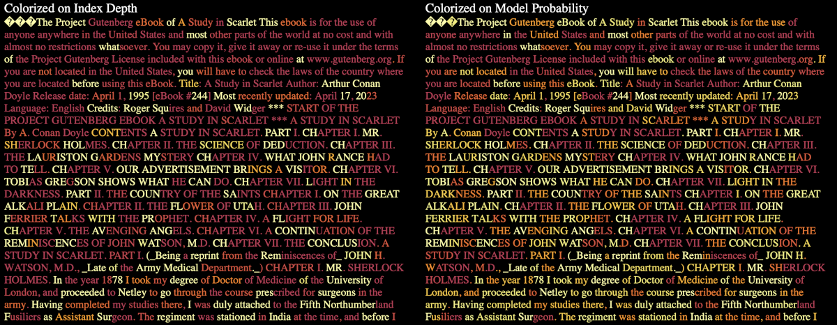
Figure 4 shows the distribution of index symbols in the compression above. As can be seen nearly 40% of tokens are predicted perfectly.

Figure 5 show a more detailed view of how and what the model predicted. It is a heat map where the color ranges from deep red for words that were easily predicted (and added little to no entropy) to white for words that were low probability and a surprise to the model, so adding much more entropy.

Generating Some Text

Decompressing uses the LLM in the same way as compression: it predicts the next possible tokens and then uses the stored data to correct that prediction, steering the output.

We could intercept this and provide the decompressor with data NOT from the statistical decoder. The module tokensOfData tokenizes the comment from the command line options and puts that at the beginning of the output symbol stream as a prompt. Then it treats its input file as a stream of 4-bit numbers and puts the associated index symbol in the output stream.

First, let's try a string of zeros to see the most likely prediction (also called the 'Zero Temperature' prediction):

% echo -n '\0\0\0\0\0\0\0\0\0\0\0\0\0\0\0\0\0\0' |\
python3.9 -m tokensOfData -n gpt2 -c 'Complete a long poem about green trees.' |\
python3.9 -m modelOfInx -n gpt2 -w 128 -cd 0.5 | python3.9 -m tokensToStr -n gpt2

Complete a long poem about green trees. I'm not sure if it's a good idea to write a poem about a tree, but I think it's a good idea to write a poem about a tree. %
%

And then we can try some random string:

% echo 'Just some randomness' |\
python3.9 -m tokensOfData -n gpt2 -c 'Complete a long poem about green trees.' |\
python3.9 -m modelOfInx -n gpt2 -w 128 -cd 0.5 |\
python3.9 -m tokensToStr -n gpt2

Complete a long poem about green trees. ******** A. Green is an old-school name which may well indicate how to grow a green plant without the roots already present and it certainly helps for that (as the plants do NOT require watering.)%
%

Which is not too bad for raw GPT-2 output.

However, ASCII text is not a good source of randomness. If we want to stick with a human-readable random string, we could do better by compressing the input to squeeze out redundancy, making every bit equally relevant. We could do better still if the input data was not used as a flat 4-bit selection but fed through, say, an entropy decoder to give index symbols that match a desired distribution. But that's an example for another time!

From these two examples, it should be clear that an LLM text generator is just extending a string by adding some amount, often zero, of entropy to the string symbol by symbol.

If we recompress either of these examples, we get back exactly the string we put in: zeros in the first example and 4-bit numbers in the second. In both cases, there are no surprises for the model, and the entropy in the text after the prompt is very low, indicating that the text was likely LLM-generated.

It should also be clear that this is an entirely deterministic process: we can push the information in any text toward a raw entropy representation by 'compressing,' or any entropy toward something human-readable by 'decompressing.' Chatbot LLMs work by using a random number generator for the entropy, although obviously, they are not factored into a decompressor like I've done here.

Conclusion

So, our exploration into using LLMs as predictive models within a compression framework offers a subtly different perspective on how these models generate text. By framing an LLM’s output through the lens of compression, we can see that generating text is not really a process of random word selection but a sophisticated extension of a prompt with controlled entropy. It is this controlled addition of entropy that allows LLMs to produce coherent and contextually relevant text that often feels creatively inspired.

Exactly why LLMs are such good predictors - well that's a whole different article!

TODO

• I'd like to run the scripts against GPT-3.5-turbo, GPT-4, and the LLaMA models to see how much better they do and maybe come up with a benchmark score to compare them.

• I'd also like to add some heat maps of generated texts from these models to show the low recognizable entropy distributions compared to human-generated text. GPT-2 generated text isn't very good to start with, and the maps were hard to read, making them not good examples of the technique.

• I should fill out the last example by using the .bin data from one compression as the entropy for generating text. This would be a filter that removed the unpredicted tokens and treats all the data as if it were indices with a new distribution. Recompressing this generated text would reproduce the original .bin file, which could then be decompressed to recover the original message. With a little more work, this might be an interesting steganographic tool.

• Neural nets are generic function approximators. I'd like to train a small net using the Martian pressure data and see if I can recover the two-sine wave approximation from what it learned, and then close the loop by building the compressor with that learned predictive model at its core.